レイトレ合宿8アドベントカレンダーの最初の週の投稿です。 またGraphics Programming weekly に紹介されました!
The first week's Raytracing Camp 8 advent calendar post. Graphics Programming weekly featured this article!
このブログ投稿では、魔方陣から始まり、群論、QMC、そして最後にレイトレのサンプラーの話をします。
In this blog post, I start with the magic square, then move on to group theory, QMC, and finally, a sampler of raytracing.
魔方陣、ガロア体、QMC(Magic square, Glois field, QMC)

TL;DR
この投稿の要約は以下の通りです。
- 魔方陣を機械的に構成する方法について述べ、大きなサイズ、また高次元に拡張します。
- 魔方陣を拡張するために群論について触れます。
- QMCについて軽く触れます。
- 魔方陣を使った新しいサンプラーを紹介します。
- 他の手法との簡単な比較を行います。
最終的に次のようなプロットのサンプラーを得ます。
A summary of this post follows.
- I will discuss how to construct a magic square mechanically and extend it to larger sizes and higher dimensions.
- I will discuss group theory in order to extend the magic square.
- QMC will be briefly discussed.
- A new sampler using magic square will be introduced.
- A brief comparison with other methods.
Finally, we build the sampler that plots the following.
魔方陣(Magic square)
ここに、3x3のマスの中に1から9までの数字が入ったものがあります。
Here is a 3x3 square with numbers from 1 to 9 in it.
| 6 | 1 | 8 |
| 7 | 5 | 3 |
| 2 | 9 | 4 |
このとき、どの行、どの列の和も15になっています。
例えば1行目は、6+1+8=15
例えば2列目は、1+5+9=15
確かに15になっています。
これを3x3の 魔方陣 と呼びます。魔"法"陣ではなく、魔"方"陣です。注意しましょう。
驚くべきことに、実は3x3の魔方陣は回転や反転を除くとこの一種類しかありません。
同様のことを4x4でもできます。
In this case, the sum of any row or column is 15.
For example, the first row is 6+1+8=15
For example, the second row is 1+5+9=15
It is indeed 15.
This is called a 3x3 magic square.
Surprisingly, there is only one type. of 3x3 magic square except for rotation and reversal
We can do the same thing with 4x4.
| 16 | 9 | 6 | 3 |
| 5 | 4 | 15 | 10 |
| 11 | 14 | 1 | 8 |
| 2 | 7 | 12 | 13 |
4x4の場合は 880通り の組み合わせがあるそうです。
5x5の場合は 約3億通り の組み合わせがあるそうです。
3億通りもあるのならば、自分の手で適当にやっても、魔方陣を作れそうな気がします。
しかし実際にやってみると、なかなかうまいことできません(実際にやってみてください😊)。
こうなったら、何か機械的な方法で、魔方陣を作りたいという気持ちになります。
In the case of 4x4, there are 880 combinations.
In the case of 5x5, there are approximately 300 million combinations.
If there are 300 million ways to make a magic square, You think you can make it even if you do it with your own hands?
But when you actually try it, it's not so easy to get it right.
When this happens, you want to create a magic square in some mechanical way, don't you?
ラテン方陣(Latin square)
最初から一般的な大きさの魔方陣を作るのは難しそうなので、
簡単な問題、具体的には3x3の魔方陣を機械的に作る方法から攻めてみます。
唐突ですが、ここで0から2までの三つの数字を3組使って、
どの行も、どの列も0から2の数字が全て登場する方陣 を作ってみます。
この方陣を$u$と置きます。
Since it seems difficult to make a magic square of a general size from scratch,
we attack a simple problem, specifically, how to make a 3x3 magic square mechanically.
In first, using three sets of three numbers from 0 to 2,
Let's make a square in which all the numbers from 0 to 2 appear in every row and every column.
Let $u$ denote this square.
$u$
| 0 | 1 | 2 |
| 1 | 2 | 0 |
| 2 | 0 | 1 |
この方陣を ラテン方陣 といいます。
元々は数字ではなく、A,B,Cのラテン文字を使っていたことからそう言われています。
ここでこの数字の並びをもっとコンパクトに定義する方法を考えてみます。
列方向を$x$、行方向を$y$、最終的に得られる値を$u$とすると、
上のラテン方陣は、次のような一次式に対応します。
This square is called the Latin Square.
It is so-called because it initially used the Latin letters A, B, and C instead of numbers.
Here is a more compact way to define this sequence of numbers.
Let $x$ denote the column direction, $y$ the row direction, and $u$ the final value obtained.
The Latin square above corresponds to the following linear equation.
実は、ラテン方陣を構成する式は必ずこのような一次式になります 。
本当かどうか確かめてみましょう。
yを固定して考えてみると、x方向の3つの数は次の6通りしかありえず、
それぞれ右のような一次式に対応します。
The equation that makes up the Latin square is always a linear equation like this.
Let's see if it is true.
If we fix y, there can be only six possible numbers of 3 in the x-direction,
and Each corresponds to the linear equation shown on the right.
(0,1,2) $u \equiv x \pmod 3$
(0,2,1) $u \equiv 2x \pmod 3$
(1,0,2) $u \equiv 2x+1 \pmod 3$
(1,2,0) $u \equiv 1x+1 \pmod 3$
(2,0,1) $u \equiv 1x+2 \pmod 3$
(2,1,0) $u \equiv 2x+2 \pmod 3$
確かに対応していることがわかりました。
y方向も同様なので、ラテン方陣は、2変数の一次式で表現できることがわかりました。
We found that they do indeed correspond.
Since the same is true in the y-direction,
we found that the Latin square can be expressed by a linear equation in two variables.

オイラー方陣(Euler Squares)
ラテン方陣をもう一つ用意します。これを$v$とします。
We prepare another Latin square. Let $v$ denote this.
$$ v \equiv 2x + 1y \pmod 3 \\ $$$v$
| 0 | 2 | 1 |
| 1 | 0 | 2 |
| 2 | 1 | 0 |
この二つのラテン方陣$u$と$v$を、それぞれ別の桁の数字だと思って、一つにまとめると次のようになります。
If we think of these two Latin squares $u$ and $v$ as separate digits and combine them into one, we get the following.
$uv$
| 00 | 12 | 21 |
| 11 | 20 | 02 |
| 22 | 01 | 10 |
1桁目と2桁目の数のペアを一繋がりの2桁の3進数だとみなすと、
00から22までの全ての数字が出尽くしてることに気が付きます!
よりわかりやすく同じ$uv$を10進数にすると次のようになります。
If we consider the pair of first and second digit numbers to be a single connected two-digit ternary number,
we find that we have all the digits from 00 to 22!
To make it easier to understand, the same $uv$ is converted to a decimal number as follows.
$uv$(10進法,base-10)
| 0 | 5 | 7 |
| 4 | 6 | 2 |
| 8 | 1 | 3 |
0から始まっているので、各行と列の合計は12になっていますが、まぎれもなく これは魔方陣です!!
魔方陣になる前の3進数のままのものを オイラー方陣 と呼びます。
ラテン方陣をテキトーに二つ組み合わせれば、必ずオイラー方陣になるのでしょうか?
Starting from 0, the sum of each row and column is 12, but unmistakably this is a magic square!
The one that is still in ternary before becoming a magic square is called an Euler square.
Are two Latin squares always an Euler square?
$v^{\prime}$を次のように定義します。
Define $v^{\prime}$ as follows.
$ v^{\prime} \equiv 2x + 2y \pmod 3 \\ $
このとき$v^{\prime}$のラテン方陣と、$uv^{\prime}$は次のようになります。
At this point, the Latin square of $v^{\prime}$ and $uv^{\prime}$ are as follows.
$v^{\prime}$
| 0 | 2 | 1 |
| 2 | 1 | 0 |
| 1 | 0 | 2 |
$uv^{\prime}$
| 00 | 12 | 21 |
| 12 | 21 | 00 |
| 21 | 00 | 12 |
$uv^{\prime}$ (10進法,base-10)
| 0 | 5 | 7 |
| 5 | 7 | 0 |
| 7 | 0 | 5 |
合計こそ全ての行が12になっていますが、
0,5,7が3回ずつ出てしまい、代わりに1,2,3,4,6,8が現れず、魔方陣になれませんでした。
一体 $uv$がうまくいって、$uv^{\prime}$がうまくいかない理由は何なのでしょうか?
The total is 12 for all the rows, but 0,5,7 appeared 3 times each,
and 1,2,3,4,6,8 didn't appear instead, so it couldn't be a magic square.
Why can we construct a Latin square from $uv$ and not a Latin square from $uv^{\prime}$?
オイラー方陣を作れる条件 (Conditions for making an Euler square)
先ほどの$u$と$v$と$v^{\prime}$についてもう一度式を見直してみます。
うまくいく$u$と$v$は次のようになっていました。
Let's review the equations again for $u$, $v$, and $v^{\prime}$.
The $u$ and $v$ are as follows.
うまくいかない$u$と$v^{\prime}$は次のようになっていました。
The $u$ and $v^{\prime}$ are as follows.
$$ \begin{align*} u &\equiv 1x + 1y \pmod 3 \\ v^{\prime} &\equiv 2x + 2y \pmod 3 \\ \end{align*} $$方程式の$x$や$y$は毎回同じなので、係数部分だけ取り出して、それを$M$と置きます。
Since $x$ and $y$ in the equation are the same each time, we take out only the coefficient part and place it as $M$.
$$ M_{uv} = \begin{bmatrix} 1 & 1 \\ 2 & 1 \\ \end{bmatrix} $$$$ M_{uv^{\prime}} = \begin{bmatrix} 1 & 1 \\ 2 & 2 \\ \end{bmatrix} $$この時ベクトル$(u,v)$を$U$と、ベクトル$(x,y)$を$X$と、置くと次のような式になっていたということになります。
If we let the vector $(u,v)$ as $U$ and the vector $(x,y)$ as $X$, we have the following equation.
$$ U = M X $$もし逆行列$M^{-1}$が存在したら、$M^{-1}$を両辺の左からかけることで次のようになります。
If the inverse matrix $M^{-1}$ exists, multiplying $M^{-1}$ by the left of both sides of the equation.
$$ M^{-1} U = X $$これはつまり、 「$M$が逆行列を持つなら、$(u,v)$と$(x,y)$が一対一に対応する」 ということになります。
まとめるとこういう論理の流れです。
- ラテン方陣を二つ組み合わせれば、各行と各列の和は必ず等しくなる。
- ラテン方陣を二つ組み合わせても、$M$が逆行列を持たなければ全ての数字が出ない。
- つまりオイラー方陣が成り立つためには、$M$が逆行列を持たなければなりません。
確かめてみます。
This means that "If $M$ is invertible, then $(u,v)$ and $(x,y)$ are bijection".
- If two Latin square columns are combined, the sum of each row and each column is always equal.
- Even if we combine two Latin Squares, if $M$ does not have an inverse matrix, we will not get all the numbers.
- In other words, for the Euler square to be valid, $M$ must have an inverse matrix.
Let's check it out.
$$ \det M_{uv} = \det \begin{bmatrix} 1 & 1 \\ 2 & 1 \\ \end{bmatrix} = 2 \pmod 3 \\ $$$$ \det M_{uv^{\prime}} = \det \begin{bmatrix} 1 & 1 \\ 2 & 2 \\ \end{bmatrix} = 0 \pmod 3 $$確かにオイラー方陣を構成する$M_{uv}$の行列式が0になっておらず、オイラー方陣を構成しない$M_{uv^{\prime}}$の行列式は0になっています。
ちなみに、オイラー方陣を構成するラテン方陣を、直交するラテン方陣 と呼びます。
ラテン方陣を構成するための係数の行列$M$の行列式が0以外の数字であれば、
そのラテン方陣はオイラー方陣を作る ということがわかりました!
どんどん発展させていきましょう。次は4x4のオイラー方陣を作ります!
Certainly, the determinant of $M_{uv}$, which constitutes an Euler square,
is not zero, and the determinant of $M_{uv^{\prime}}$, which does not constitute an Euler square, is zero.
By the way, a Latin square that constitutes an Euler square is called a orthogonal Latin square.
If the determinant of the matrix $M$ of coefficients to form the Latin square is
a non-zero number, then the Latin square makes an Euler square!
Let's keep expanding it! Next we'll build a 4x4 Euler square!
オイラー方陣(4x4) (Euler square(4x4))
3x3で使ったものと同じ$M$を使って、mod 4の世界で行列式を計算します。
Same as used in 3x3 M to compute the determinant in the mod 4 world.
$$ \det M = \det \begin{bmatrix} 1 & 1 \\ 2 & 1 \\ \end{bmatrix} = 1 \pmod 4 $$大丈夫そうです!実際にラテン方陣を作ってみます。
It looks fine! Let's make an Latin square.
$u$
| 0 | 1 | 2 | 3 |
| 1 | 2 | 3 | 0 |
| 2 | 3 | 0 | 1 |
| 3 | 0 | 1 | 2 |
$v$
| 0 | 2 | 0 | 2 |
| 1 | 3 | 1 | 3 |
| 2 | 0 | 2 | 0 |
| 3 | 1 | 3 | 1 |
どうやら具合が悪そうな方陣ができてしまいました。
$v$は列はいいのですが、全ての行に同じ数字が二回出てしまい、ラテン方陣の要件、「全ての行と列に違う数字を出す」を満たしていません。
ぐっとにらむと、$M$の係数の2が、4の約数であることから、こういう"パターン"がでるのは必然に思えます。
何らかの数字に2を足していった数列を、mod 4の世界で見ると次のようになります。
The same number appears twice in every row and does not satisfy the Latin Square requirement.
Since the coefficient of $M$, 2, is a divisor of 4, it seems inevitable that such a "pattern" would emerge.
The sequence of numbers obtained by adding some number to some number, in a mod four world, looks like this.
0->1->2->3->0 (Loop starting from 1 and then keep adding by 3. All numbers from 0 to 3 have appeared.)
1->3->1->3->1 (Loop starting from 1 and then keep adding by 2. There are no 0 and 2 in the sequence.)
0->2->0->2->0 (Loop starting from 1 and then keep adding by 2. There are no 1 and 3 in the sequence.)
全ての数字が登場せず、長さ2の短いループでグルグル回ってしまうのがよくなさの原因です。
仮に次のようにどのような数の倍数であっても、短いループは作らずに、
必ず全ての数が登場し、長さ3のループになるような世界があったらうれしそうです。
It is impossible to create a Latin square because all the numbers do not appear and
go around in a short loop of length 2.
It would be nice to have a world where no matter what numbers you add,
they will always show up in a loop of length 3, with all the numbers appearing in that sequence.
A->C->B->A->C->B->... (Loop starting from A and then keep adding by B)
A->B->C->A->B->C->... (Loop starting from A and then keep adding by C)
B->A->C->B->A->C->... (Loop starting from B and then keep adding by C)
群論に出てくるガロア体ならそれを可能にします!
Galois fields in group theory would make that possible!

群、環、体、ガロア体(Group, Ring, Field, Galois field)
唐突ですが、群について書きます。
詳しくは 専門書を当たってほしい のですが、軽く書きます。
I explain about group theory.
For more details, please refer to a textbooks, but here is a brief description.
群(Group)
次の条件を満たす、ある集合$G$と、その集合に対する二項演算 $\cdot$ のペアを群と呼びます。
また 群の要素を元(げん) といいます。
- その二項演算の結果もまた集合$G$になる。
- 二項演算 $\cdot$ が結合法則を満たす。
- $a \cdot e = a$ となるような、その演算を行っても元が変わらない元$e$(単位元)がある。
- $a \cdot b = e $ となるような元(逆元)が存在する。
具体例をあげるとわかりやすいです。
- 自然数足す自然数は、自然数なので群です。
- 自然数掛ける自然数は、自然数なので群です。
- 自然数割る自然数は、有理数なので群ではありません。
- 自然数引く自然数は、(負も含む)整数なので群ではありません。
- 有理数掛ける有理数は、有理数なので群です。
などなど...
A pair of a set $G$ and a binary operation $\cdot$ on that set that satisfies the following conditions is called a group.
- The result of that binary operation is also a set $G$.
- The binary operation $\cdot$ satisfies the join rule.
- There is a $e$ whose element does not change after that operation such that $a \cdot e = a$.
A concrete example is easy to understand.
- Natural number + natural number is a group because result is a natural number.
- Natural number x natural number is a group because result is a natural number.
- Natural number/natural number is not a group because result is a rational number.
- Natural number - natural number is not a group because result is an integer (including negative numbers).
- Rational numbers x rational numbers are rational numbers and therefore a group.
etc...
環(Ring)
群の種類に、"環(かん)" というものがあります。環となるには次の要件を満たさないといけません。
- 結合法則が成り立つ演算$+$がある。加法といい、足し算みたいなものです。
- 分配法則が成り立つ演算$\cdot$がある。乗法といい、掛け算みたいなものです。
具体例をあげると次のようなものです。
- 有理数は、足し算、掛け算が成り立ち、結合法則も分配法則も成り立つので環です。
- 法が6の時の合同式は、足し算、掛け算が成り立ち、結合法則も分配法則も成り立つので環です。
これでこの歌詞の意味が分かるようになりました。
There is a type of group called a "ring". To be a ring, it must satisfy the following requirements
- There is an operation $+$ for which the associative property holds.
- There is an operation $\cdot$ for which the Distributive property holds.
Specific examples are as follows.
- Rational numbers are rings because they can be added and multiplied, and both the join rule and the distributive law hold.
- A congruence when the law is 6 is a ring because addition and multiplication hold, and both the join and distribute rules hold.
Now you know what these lyrics mean.
体(Field)
環に加えて、乗法に関する逆元、つまり掛け算したら、割ったみたいになるものが元の中にあったら、それは 体 です。
具体例をあげると次のようなものです。
- 有理数は通常の加算乗算ができ、乗法に関する逆元があるので体です。例えば、1.25の乗法に関する逆元は0.8です。
- a,bを有理数としたとき、a+b $\sqrt{2}$ の集合は体です 。不思議ですね。
In addition to rings, if there is an inverse element related to multiplication,
i.e., something in the original that, when multiplied, makes it look like it is divided, then it is a field.
Specific examples are as follows.
- Rational numbers are field because they can be multiplied by ordinary addition and have inverses regarding multiplication.
For example, the inverse with respect to multiplication of 1.25 is 0.8. - When a and b are rational numbers, the set a+b $\sqrt{2}$ is a field.
有限体
お疲れ様です! やっと有限体に来ました。ここから楽しくなってきます。
有限体とは、元(集合の要素)の個数が有限な体です。
え、それだけ?と思われるかもしれませんが、ここでとても不思議なことが起きます。
なんとこれまで出てきた定義だけで、元の数を決めると有限体は一種類に決まってしまうのです!
有限体は、エヴァリスト・ガロア(Évariste Galois)が発見したので、ガロア体とも呼ばれます。
元の個数を$q$とするとそのガロア体は$GF(q)$や$F_q$の様な書き方をします。$q$を位数と呼びます。
また$q$は任意の数字は取れず、素べき(素数のべき乗)の時のみガロア体は構成できます。
Congrats! It' s finally here at the finite field. This is where the fun starts.
A finite field is a field with a finite number of elements.
Oh, that's it? You may think, But here is a very mysterious thing.
What a surprise, with only the definitions we've come up with so far,
Once the number of elements is determined, the finite field will be one type!
Finite field is also called Galois field because that is discovered by Évariste Galois.
If the number of elements is $q$, its Galois field is written like $GF(q)$ or $F_q$. We call $q$ the order or size.
有限体、もといガロア体(Finite field, Galois field)
ガロア体の演算結果を導くのは中々大変なのと、レイトレを書いている人にはあまり興味がない かもしれないので、
具体的な演算方法はここには書かきませんが、ご興味のある方は最後に書いてある参考書籍をあたってください。
ガロア体の演算結果を導くのは大変ですが、演算結果自体は元が有限なので小さな表に収まります。
例えば、元の数が4個の時、つまり$GF(4)$の時の加法と乗法は次のようになります。
It isn't easy to derive the result of a Galois, and it may not be of interest to people who are writing ray tracing.
If you are interested, please refer to the reference books mentioned at the end of this article.
Deriving the result of a Galois is hard, but the result itself fits into a small table because the number of elements is finite.
For example, when the order is 4, i.e. $GF(4)$, the addition and multiplication are as follows.
加算表(Addition)
| + | 0 | 1 | 2 | 3 |
| 0 | 0 | 1 | 2 | 3 |
| 1 | 1 | 0 | 3 | 2 |
| 2 | 2 | 3 | 0 | 1 |
| 3 | 3 | 2 | 1 | 0 |
乗算表(Multiplication)
| x | 0 | 1 | 2 | 3 |
| 0 | 0 | 0 | 0 | 0 |
| 1 | 0 | 1 | 2 | 3 |
| 2 | 0 | 2 | 3 | 1 |
| 3 | 0 | 3 | 1 | 2 |
この表を 群表 と呼び、全ての演算結果 がこの表に収まります。
この結果はWolfram Alphaでも確認できます。
Wolfram Alpha上では(0,1,a,b)という表記になっていますが、これは上の表と別のものを表しているわけではなく、
まったく同じものを表しています!。数字自体にあまり意味がないからこのような表記が可能なのです。
例えば、(⭕,🔺,🔳,❌)でも群は定義できて、乗算表は次のようになります。
All results of all operations fit into this table.
This result is also available on Wolfram Alpha.
On Wolfram Alpha, the notation (0,1,a,b) does not represent something different from the table above,
but exactly the same thing. This is possible because the numbers themselves don't have any meaning.
For example, (⭕,🔺,🔳,❌) can also define a group and the addition and multiplication table would look like this.
加算表(Addition)
| + | ⭕ | 🔺 | 🔳 | ❌ |
| ⭕ | ⭕ | 🔺 | 🔳 | ❌ |
| 🔺 | 🔺 | ⭕ | ❌ | 🔳 |
| 🔳 | 🔳 | ❌ | ⭕ | 🔺 |
| ❌ | ❌ | 🔳 | 🔺 | ⭕ |
乗算表(Multiplication)
| x | ⭕ | 🔺 | 🔳 | ❌ |
| ⭕ | ⭕ | ⭕ | ⭕ | ⭕ |
| 🔺 | ⭕ | 🔺 | 🔳 | ❌ |
| 🔳 | ⭕ | 🔳 | ❌ | 🔺 |
| ❌ | ⭕ | ❌ | 🔺 | 🔳 |
さきほど長さが短いループが作られてしまうからラテン方陣が作れないという話をしました。
ガロア体で、加算が小さなループを作っていないかを見てみます。
Earlier I mentioned that we can't make a Latin square because it would create loops of short length.
Let's look at Galois and see if the addition does not create small loops.
🔺-> ❌ -> 🔳 -> 🔺-> ❌ -> 🔳 ->... (Loop starting from 🔺 and then adding by 🔳)
🔺-> 🔳 -> ❌ -> 🔺-> 🔳 -> ❌ ->... (Loop starting from 🔺 and then adding by ❌)
🔳-> 🔺 -> ❌ -> 🔳-> 🔺 -> ❌ ->... (Loop starting from 🔳 and then adding by ❌)
すべて長さ3のループになっています!
小さな表に収まるという性質は ソフトウェア開発の観点からもうれしいこと です。
なぜなら小さな二次元配列のテーブルに群表を格納して、
ガロア体の上で計算する場合はそのテーブルから値を参照するだけでよいからです。
またPythonであればgaloisという、ガロア体を扱うライブラリがありこれを使うのが便利です。
このライブラリを使って実際に群表を作ってみたものが次のコードです。
All loops have a length of 3!
The property of being able to fit into a small table is a nice thing for software engineering.
This is because we can store the table in a small two-dimensional array table and
then simply refer to values from that table when computing on Galois field.
In Python, it's convenient to use galois, a library that handles Galois field.
The following code shows a table created using this library.
# 群表を作る
import galois
import numpy as np
#
def plotTable(op,opstr):
    #
    q  = 4
    GF = galois.GF(q)
    #
    print(opstr,end=' ')
    for i in range(q):
        print(i,end=' ')
    print('')
    #
    for i in range(q):
        print(i, end=' ')
        for j in range(q):
            print(np.copy(op(GF(i),GF(j))), end=' ')
        print('')
    print('')

plotTable(lambda a, b: a + b, '+')
plotTable(lambda a, b: a * b, 'x')
$q$が素べき($2^5$とか$3^4$とか)でなく、素数($5$とか$11$とか)であれば、単なるmodの計算と同じになります。
例えば、$GF(5)$は次のようになります。
It is the same as just computing mod if $q$ is a prime number (like $5$, $11$) instead of a prime power (like $2^5$, $3^4$).
For example, $GF(5)$ looks like this.
加算表(Addition)
| + | 0 | 1 | 2 | 3 | 4 |
| 0 | 0 | 1 | 2 | 3 | 4 |
| 1 | 1 | 2 | 3 | 4 | 5 |
| 2 | 2 | 3 | 4 | 0 | 1 |
| 3 | 3 | 4 | 0 | 1 | 2 |
| 4 | 4 | 0 | 1 | 2 | 3 |
乗算表(Multiplication)
| x | 0 | 1 | 2 | 3 | 4 |
| 0 | 0 | 0 | 0 | 0 | 0 |
| 1 | 0 | 1 | 2 | 3 | 4 |
| 2 | 0 | 2 | 4 | 1 | 3 |
| 3 | 0 | 3 | 1 | 4 | 2 |
| 4 | 0 | 4 | 3 | 2 | 1 |
ループの長さも常に4になります。
The length of the loop is always four as well.
1->4->2->0->3->1 (Loop starting from 1 and then adding by 3)
2->4->1->3->0->2 (Loop starting from 2 and then adding by 2)
4->2->0->3->1->4 (Loop starting from 4 and then adding by 3)
これは素数が、それよりも小さい数と常に互いに素であるから成り立つわけです。
素べきではなく、素数を使えば、小さなテーブルすら不要です。
This is possible because prime numbers are always coprime with lesser numbers.
If we use prime numbers instead of prime powers, we do not even need that small table.
オイラー方陣(4x4) 再挑戦
何をしていたのか忘れそうなのでいったんまとめます。
- 魔方陣(オイラー方陣)を拡張したい
- 3x3のオイラー方陣は、3を法にして、ラテン方陣から作れた
- 4x4のオイラー方陣は、4を法にしても、ラテン方陣を作れない
当然ここからの流れは、
「4x4のオイラー方陣は、位数4のガロア体 $GF(4)$を使って作ったラテン方陣から作れる!」
です。
3x3の場合と同じ$M$を使って、$GF(4)$の世界で行列式を計算します。
群表を見返し、整数だと思って計算してしまう癖に注意しながら計算してみます。
I'll summarize because we seem to forget what we were doing.
- We want to extend the magic square (Euler square)
- 3x3 Euler square can be made from the Latin square by mod 3.
- 4x4 Euler square can't be made from Latin square in mod 4 world.
Of course, here's where things go from here.
"A 4x4 Euler square can be made from a Latin square made from a $GF(4)$!"
Calculate the determinant in the $GF(4)$ world using the same $M$ as in the 3x3 case.
Calculate using the table from before. Be careful not to think of it as an normal integer.
まずは行列式は大丈夫そうです!
ラテン方陣を作ってみます。
The determinant looks fine!
Let's make a Latin square.
$u$
| 0 | 1 | 2 | 3 |
| 1 | 0 | 3 | 2 |
| 2 | 3 | 0 | 1 |
| 3 | 2 | 1 | 0 |
$v$
| 0 | 2 | 3 | 1 |
| 1 | 3 | 2 | 0 |
| 2 | 0 | 1 | 3 |
| 3 | 1 | 0 | 2 |
大丈夫そうです!最後にオイラー方陣を作ってみます。
It looks fine! Finally, we'll try to make an Euler square.
$uv$
| 00 | 12 | 23 | 31 |
| 11 | 03 | 32 | 20 |
| 22 | 30 | 01 | 13 |
| 33 | 21 | 10 | 02 |
$uv$(十進数)
| 0 | 6 | 11 | 13 |
| 5 | 3 | 14 | 8 |
| 10 | 12 | 1 | 7 |
| 15 | 9 | 4 | 2 |
ついにやりました! これで4x4の魔方陣が機械的に作れるようになりました!
これまでは2次元の魔方陣でしたが、次は3次元の魔方陣が作りたくなってきます。
もちろんガロア体を使って作ります!
We finally did it! Now we can mechanically create a 4x4 magic square!
It has been a 2-dimensional magic square, but now I want to make a 3-dimensional magic square.
Of course, We will make it using Galois field!

オイラー方陣(4x4x4) (Euler Square(4x4x4))
これまでは2変数の1次式を2つ使って、桁数が2、次元が2のオイラー方陣を作ってきました。
ここからは3変数の1次式を3つ使って、桁数が3、次元が3のオイラー方陣を作ります。
早速具体的な$M$を出すと、次のような$M$であれば3次元のオイラー方陣が作れます。
So far, we have used two two-variable linear expressions to create an Euler square with two digits and two dimensions.
We will use three three-variable linear expressions to create an Euler square with three digits and three dimensions.
For example, the following M can be used to create a three-dimensional Euler square.
$$ M = \begin{bmatrix} 2 & 1 & 1 \\ 1 & 2 & 1 \\ 1 & 1 & 2 \\ \end{bmatrix} $$確認のため$GF(4)$で$\det M$を計算してみます。
Let us calculate $\det M$ with $GF(4)$ for confirmation.
$$ \det M = \det \begin{bmatrix} 2 & 1 & 1 \\ 1 & 2 & 1 \\ 1 & 1 & 2 \\ \end{bmatrix} = 2 $$大丈夫そうです。
実際に3次元のオイラー方陣を、作ったのが次の表です。
2次元の表で表すために、Zを固定した表を三つに分けて書いています。
確かにどの行も列もZ方向も、各桁の数字にが重複なく、全体からみてもそれぞれの数字は一意になっています!
It looks okay.
The following table shows the actual 3-dimensional Euler square.
To represent it in a 2-dimensional table, we have divided the table into three parts with fixed Z.
Indeed, each digit in every row, column, and Z direction has no duplicates, and each digit is unique!
z = 0
| 000 | 211 | 322 | 133 |
| 121 | 330 | 203 | 012 |
| 232 | 023 | 110 | 301 |
| 313 | 102 | 031 | 220 |
z = 1
| 112 | 303 | 230 | 021 |
| 033 | 222 | 311 | 100 |
| 320 | 131 | 002 | 213 |
| 201 | 010 | 123 | 332 |
z = 2
| 223 | 032 | 101 | 310 |
| 302 | 113 | 020 | 231 |
| 011 | 200 | 333 | 122 |
| 130 | 321 | 212 | 003 |
z = 3
| 331 | 120 | 013 | 202 |
| 210 | 001 | 132 | 323 |
| 103 | 312 | 221 | 030 |
| 022 | 233 | 300 | 111 |
このオイラー方陣をコードで表現してみます。
Let us try to express this Euler square in code.
# 4x4と4x4x4のオイラー方陣を構成する
import numpy as np
import galois

# 4x4の例
q  = 4
GF = galois.GF(q)
M = GF([[1,1],[2,1]])
for y in range(q):
    for x in range(q):
        r = np.copy(np.matmul(M,GF([x,y])))
        print(f'{r[0]}{r[1]}', end=' ')
    print('')
print('')

# 4x4x4の例
q  = 4
GF = galois.GF(q)
M = GF([[2,1,1],[1,2,1],[1,1,2]])
for z in range(q):
    for y in range(q):
        for x in range(q):
            r = np.copy(np.matmul(M,GF([x,y,z])))
            print(f'{r[0]}{r[1]}{r[2]}', end=' ')
        print('')
    print('')
これも問題なく動いていることを確認できました。
4x4x4のオイラー方陣をコードで作ることに成功しました!
3次元が作れるようになったので、当然4次元のオイラー方陣も作りたくなってきます。
I can confirm that this is also working fine.
We have successfully created a 4x4x4 Euler square in code!
Now that we can make a 3-dimensional Euler square, we naturally want to make a 4-dimensional Euler square.
オイラー方陣($4^4$,$4^5$,....) (Euler Square($4^4$,$4^5$,....))
$4 \times 4 \times 4 = 4^3$のオイラー方陣に使われていた$M$は次のようなものでした。
The $M$ used for the Euler square of $4 \times 4 \times 4 = 4^3$ is as follows.
$$ M = \begin{bmatrix} 2 & 1 & 1\\ 1 & 2 & 1\\ 1 & 1 & 2\\ \end{bmatrix} $$これと同じような形をした新しい$M$を次のように定義します。
We define a new $M$ with a similar form as follows.
$$ M = \begin{bmatrix} 2 & 1 & 1 & 1\\ 1 & 2 & 1 & 1\\ 1 & 1 & 2 & 1\\ 1 & 1 & 1 & 2\\ \end{bmatrix} $$これの行列式は以下の通りです。
The determinant of this is as follows.
$$ \det M = \det \begin{bmatrix} 2 & 1 & 1 & 1\\ 1 & 2 & 1 & 1\\ 1 & 1 & 2 & 1\\ 1 & 1 & 1 & 2\\ \end{bmatrix} = 3 $$この$M$は4次元のオイラー方陣を作れることになります。
どんどん拡張させて5次元、6次元のバージョンも作ってみます。
This $M$ will allow us to create a 4-dimensional Euler square.
We will continue to extend it to make 5 and 6-dimensional versions.
これもうまくいってしまいました。
この$M$は5次元のオイラー方陣を作れることになります。
うまくいきすぎていて怖いですが、いくらでも次元を増やしていけそうです。
※ 実はこの$M$は使いません。よりよい性質をもった$M$の作り方を後述します。
This also worked out well.
This $M$ will allow us to create a 5-dimensional Euler square.
I'm afraid it works too well, but I'm sure I can add as many dimensions.
※ We do not use this $M$. We will discuss later how to make $M$ with better properties.
MCとQMC
ここまで、魔方陣、ラテン方陣、オイラー方陣、群論、ガロア体、そして魔方陣の高次元化について書いてきました。
しかし、これはレイトレアドベントカレンダーなので、レイトレの話をしないといけません。
レイトレの話につなげるために、MC(Monte Carlo、モンテカルロ)法と、QMC(Quasi-Monte Carlo、準モンテカルロ)法の話を書きます。
So far, I have written about the magic square, the Latin square, the Euler square, group theory, Galois field, and the higher dimensions of the magic square.
But this is a raytracing advent calendar, so we have to talk about raytracing.
To connect this to the Raytracing story, I will explain about the MC (Monte Carlo, Monte Carlo) method and the QMC (Quasi-Monte Carlo, Quasi-Monte Carlo) method.
MC法とは、ざっくりいうと、
「ある関数$f(x)$の積分値を求めるために、$x$をランダムに決めて、$f(x)$を何回も計算して、平均する」
というものです。モンテカルロレイトレーシングの場合、$f$の積分値が画像のピクセルの値になります。
The MC method is, roughly speaking,
"To find the integral of a function $f(x)$, we randomly determine $x$, compute $f(x)$ many times and average them."
In the case of Monte Carlo ray tracing, the integral value of $f$ is the value of a pixel in the image.
ランダムと聞くと、満遍なく隅から隅までの値を返してきてくれそうなイメージがありますが、
それまでの結果と相関があったらランダムではないので、思った以上に偏ります 。
When you hear the word "random," you'd think it would return values from all corners of the spectrum, but
If there is a correlation with the previous results, it is not random, and will be more "biased" than you think .
次の図は2次元上の座標$x$をランダムにとった点の集まりの図です。
$x$を決めて$f(x)$を計算することをサンプルするというのですが、
サンプルする点がまだらになっており、すき間がところどころにあることが見て取れます。
The following figure shows a collection of points in two dimensions with coordinates $x$ taken randomly.
Determining $x$ and calculating $f(x)$ is called "sampling".
You can see that the points to be sampled are unevenly distributed, and there are gaps here and there.

これは現実世界では次のような話につながります。
これらの話のように、想像よりも低い確率になるのは、"ランダム" が思ったより"偏っている"ため です。
This leads to the following tale in the real world.
- If a coin toss continues to turn up backward, there is still a 50% chance that the next coin toss will turn up heads.
- If you draw 1000 times for a lottery ticket that has a probability of 1/1000, the probability of winning is 63%

一方でQMC法とは、ざっくりいうと、
「ある関数$f(x)$の積分値を求めるために、$x$を意図的に狙って決めて、$f(x)$を何回も計算して、平均する」
というものです。
上の図がQMCでサンプルしたものなのですが、ランダムにはなかった、すき間を積極的に塞いでいくように点がおかれているのがわかると思います。
このQMCの世界では、コイントスで裏が続いたら、次に表が出る可能性は上がり、
1/1000の確率で当たるクジを1000回引いたら大体1回当たるようになります。
こちらのほうがMC法よりも積分が素早く正確な値になりそうですよね。
具体的なQMCのアルゴリズムは無数にあり、有名なものだと以下のものがあります。
The QMC method, on the other hand, is, roughly speaking,
"To find the integral value of a function $f(x)$, we deliberately aim at $x$ to determine it, compute $f(x)$ many times, and average them."
The figure above is samples from the QMC.
You can see that the dots are placed in such a way as to actively close the gaps, which is not the case in the random case.
If the coin toss continues to show back-to-back, the likelihood of the following coin toss showing the front increases, and
If you draw a lottery ticket 1,000 times with a 1/1000 chance of winning, you will win roughly once.
It seems that the integral would be quicker and more accurate here than in the MC method.
There are many QMC algorithms, and some well-known ones include the following.
- Halton sequence
- Hammersley Point Set
- Sobol sequence
- Niederreiter sequence
- Fibonnacci Lattice
- Faure sequence
- R2 sequence
これまで作ってきた魔方陣構築方法をこのQMCに応用してみましょう!
つまり次のような置き換えをします。
- 魔方陣の番号 = サンプルのインデックス
- 魔方陣の番号がある場所 = サンプルの場所
魔方陣には、数字を入れる箱があり、(当たり前ですが)その全ての箱に数字が入っており、
隙間なく埋まっているという点で、QMCの用途にぴったりな気がします!
箱を層とここから呼びます。
Let's apply the magic square construction to QMC!
In other words, we find the following relationship between the magic square and the QMC
- Magic square number = sample index
- Location of the number = Location of the sample
The magic square has boxes for numbers, and (of course) all of those boxes have numbers in them,
and they're filled without gaps, which seems like a perfect fit for the QMC's use!
The box is called a stratum from here.
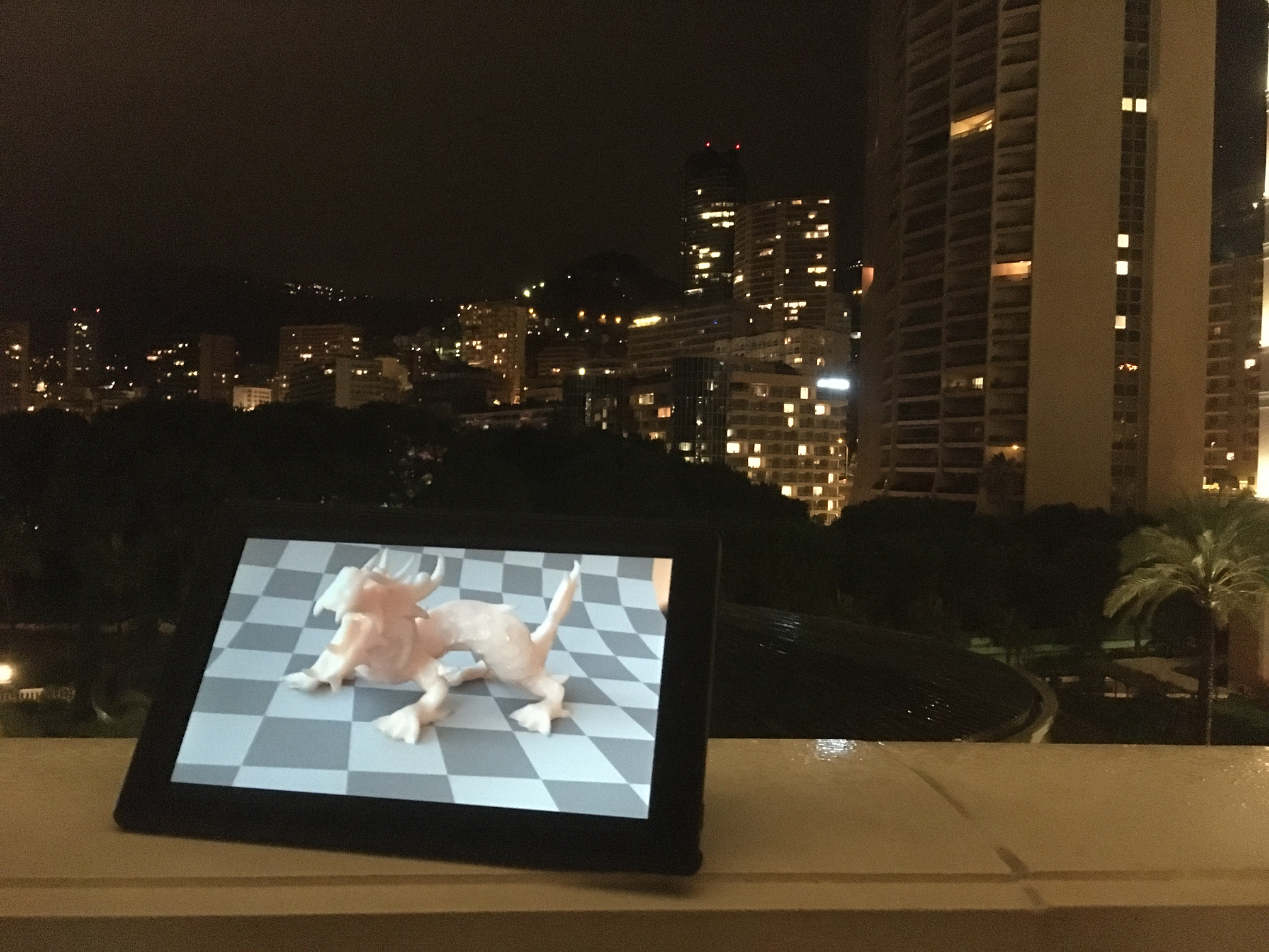
余談ですが、この写真は、モナコ公国のモンテカルロにて、モンテカルロ法の実験を行ったときの写真です。
やはりモンテカルロ法の名の由来の地だけあって、MCノイズが全く見当たりません。収束が東京のそれとは全く違いました。
レイトレ合宿8の開催場所である沖縄は東京よりもモンテカルロに(たしか)近いので同様の効果が期待できます。
By the way, the photo above shows the Monte Carlo method in Monte Carlo, Principality of Monaco.
魔方陣サンプラー(Magic Square Sampler, MSS)
まだ書いていない実装に必要な要素があるのですが、まずは先に新しいQMCサンプラーの実装とその結果を示します。
以下のコードは、魔方陣をQMCに応用したMagic Square Samplerを実装しているMSSamplerクラスと
得られたサンプル($x$のこと)をプロットする関数です。
There are elements necessary for implementation that I have not yet written, but first, I will show the implementation of the new QMC sampler and its results.
The code below is the MSSampler class that implements the Magic Square Sampler, which applies magic square to QMC, and the function that plots sample (that is $x$ ).
# サンプルをプロットする関数
# Function to plot samples
import math
import numpy as np
import matplotlib.pyplot as plt

#
def plotStairs(samples, savefile = None):
    #
    samples   = np.array(samples).T.tolist()
    numDim    = len(samples)
    numSample = len(samples[0])

    dims = []
    for d0 in range(numDim-1):
        for d1 in range(d0+1, numDim):
            dims.append([d0,d1])

    bs = 20.0
    fig = plt.figure(figsize=(bs * (numDim+1)/numDim, bs))
    #
    ps = int(2000.0/(math.sqrt(numSample)*numDim))

    for dim in dims:
        d0 = dim[0]
        d1 = dim[1]
        axPlot = fig.add_subplot(numDim, numDim+1, d0 + 1 + (d1-1) * (numDim+1))
        #
        axPlot.set_xlim(0,1)
        axPlot.set_ylim(0,1)
        #
        major_ticks = np.arange(0, 1, 1/4)
        axPlot.set_xticks(major_ticks)
        axPlot.set_yticks(major_ticks)
        axPlot.grid(which='both')
        axPlot.tick_params(
            labelleft=False, labelbottom=False,
            bottom=False, left=False,right=False,top=False)
        #
        axPlot.set_aspect('equal', 'box')
        axPlot.invert_yaxis()
        #
        if d0 == 0:
            axPlot.set_ylabel(str(d1+1))
        if d1 == numDim-1:
            axPlot.set_xlabel(str(d0+1))
        axPlot.scatter(samples[d0], samples[d1], c=range(len(samples[d1])), s=ps)

    #
    plt.subplots_adjust(wspace=0.1, hspace=0.1)
    if savefile != None:
        plt.savefig(savefile)
    plt.show()
# Magic Square Sampler
import numpy as np
import galois
#
class MSSampler:
    def __init__(self,iM,q):
        self.w  = len(iM[0])
        self.q   = q
        self.GF  = galois.GF(q)
        self.iM  = self.GF(iM)

    # IDから座標を返す
    # Return coordinates from ID
    def sample(self,id):
        digits = []
        for i in range(self.w):
            digits.append(id % self.q)
            id //= self.q
        return np.matmul(self.iM, self.GF(digits))

#
def plotMS(iM, q, ns):
    s = MSSampler(iM, q)
    samples = []
    for id in range(ns):
       x = s.sample(id)
       x = np.copy(x)
       x = (x + 0.5) / q
       samples.append(x)
    plotStairs(samples)

#
iM = [
      [1,1,1,1,1],
      [1,2,1,1,1],
      [1,3,2,1,1],
      [1,4,2,2,1],
      [1,5,3,2,2],
      [1,6,5,2,3],
      [1,7,6,3,7],
      [1,8,7,8,14],
    ]
plotMS(iM=iM, q=16, ns=16**2)

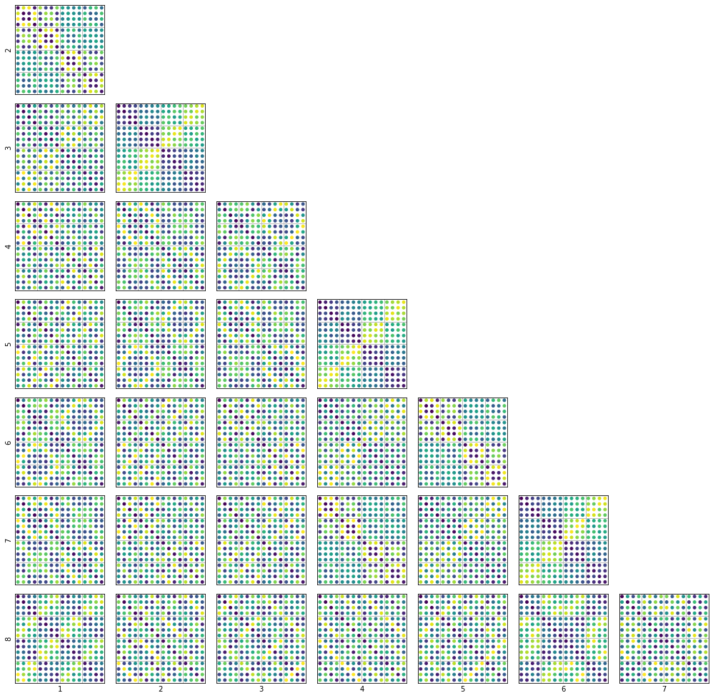
みっちり詰まっていることが伝わるでしょうか。
先のQMCの話から想像できるように、サンプルがよりみっちり詰まれば詰まるほど、積分の素早く正確な値になるため、好ましい性質があるといえます。
プロットの読み方としては、まずそれぞれの小さなプロットが、ある2次元(次元A,次元B)への投影 です。
今回のサンプルは8次元で、そのうちの2次元への投影なので、${}_8 C_2 = 28$ 個のプロットがあります。
2次元のプロットしかしていませんが、このコードは 5次元まで層化します 。
また今までは魔方陣の中にあるのは数字でしたが、点が増えると文字は見づらいので、数字を色に対応させています。
MSSampler.sample()が実装の本体ですが、たった6行しかない ことに注目してください。
Can you feel that it is tightly packed?
As you can imagine from the previous discussion of QMC, the more tightly packed the sample is,
the quicker and more accurate the integral will be, which is a desirable property.
To read the plots, first, each small plot is a projection to some two dimensions (dimension A, dimension B).
Since our sample has 8 dimensions and the projection to 2 of them, there are ${}_8 C_2 = 28$ plots.
Although only a 2-dimensional plot, this samples stratifies up to 5 dimensions.
Also, until now, it is numbers that are in the magic square,
but since letters are hard to see when there are more dots, we have made the numbers correspond to colors.
MSSampler.sample() is the core of the implementation, but notice that it has only six lines.
他の有名なサンプラーとの比較
他の有名どころのサンプラーで、MSと同程度の簡素さな実装のものたちと比較してみます。
まずはHaltonをプロットします。
Let us compare it with other well-known samplers with a similarly simple implementation to MS. First, plot Halton.
def plotSampler(sampleFun, N, maxDim):
    samples = []
    for id in range(N):
        sample = []
        for dim in range(maxDim):
            sample.append(sampleFun(id,dim))
        samples.append(sample)
    plotStairs(samples)

# Halton, RadicalInverse
def ri(id, dim):
    base = [2,3,5,7,11,13,17,19,23,29][dim]
    nume = 0
    deno = 1
    while id > 0:
        nume = nume * base + (id % base)
        deno = deno * base
        id //= base
    return float(nume) / float(deno)

plotSampler(ri, 19*17, 8)

右や下がより高次元のペアなのですが、右や下に行くほど、何らかの パターンが見えてくる のがわかると思います。
このパターンがレンダリング結果には、模様のようなアーティファクトとして現れます。
世間一般ではHaltonを直接使うことはあまりなく、これに対してスクランブル(Owen Scramblingなど)をしたり、
性質の良い上の方のプロットを何回も使いまわしたり(Padding)して、使い勝手を良くしています。
次にR2をプロットします。
The right and bottom are higher dimensional pairs, but you will notice that the further to the right and down you go, the more you will see some pattern.
This pattern appears as a pattern-like artifact in the rendered result.
Halton is not often used directly but rather scrambled (e.g., Owen Scrambling) against it in typical usage.
The upper plots with good properties are used repeatedly (padding) to make them more usable.
Next, plot R2.
# R2。8次元固定
def R2(id,dim):
	g = 1.0850702454914509
	s = 1.0/pow(g,dim+1)
	return (0.5 + s * id) % 1.0

plotSampler(R2, 512, 8)

R2もまた、サンプルされていない空間が生まれてしまっているのがわかります。
ここからは、Magic Square サンプラーの実装の詳細に入っていきます。
We can see that R2 has also created an unsampled space.
We will now go into the details of the implementation of the Magic Square sampler.
実装詳細 1.IDから座標を出す
モンテカルロレイトレでのサンプラー(変数名はsampler)は次のようなスタイルで使われます。
The sampler (variable name sampler) in Monte Carlo ray tracing is often used in the following style.
for pixel in allPixels:
    for id in range(numSamples):
        ray = createPrimalyRay()
        Le = 0
        beta = 1.0
        sampler.start(id)
        for bounce : range(maxBounce):
            R = ray.bsdf.evalBSDF(sampler.get2D())
            E = selectLight(sampler.get1D()).eval(ray.bsdf, sampler.get2D())
            Le += beta * E
            beta *= R
            ray = createSecondaryRay()
        pixel += Le
つまり、サンプルの番号が先に決まり、その後、次元を低次元の方から消費していくような形が多いと思います。
サンプルの位置が決まってから、サンプルの番号を得るわけではありません。
先述した、オイラー方陣が作れる条件のところで、次のような式を示していました。
In other words, the sample index is determined first, and then the dimensions are consumed from the lowest dimension.
The sample index is not obtained after the sample location is determined.
The following equation is shown in the previously mentioned conditions under which we can make an Euler square.
$$ M^{-1} U = X $$$U$は番号を$q$進数であらわした時の各桁の数字をベクトルにしたもので、$X$は座標です。
サンプラーを実装するにあたっても、$X$を$U$から求めるこの形になっているとうれしいわけです。
つまり$M$は不要で逆行列$M^{-1}$だけがあればいいわけです。
$U$ is a vector of the digits of the number in $q$ decimal notation, and $X$ is a coordinate.
Implementing the sampler is also good if $X$ is obtained from $U$ in this form.
In other words, $M$ is not needed. Only the inverse matrix $M^{-1}$ is required.
# MSSampler.sample()
def sample(self,id):
    digits = []
    for i in range(self.w):
        digits.append(id % self.q)
        id //= self.q
    digits = self.GF(digits)
    return np.matmul(self.iM, digits)
上のコードはMSSamplerクラスのsample関数です。
コードにも$M$が登場せず、その逆行列$M^{-1}$(変数名はiM)のみがコードにあります。
The code above is a sample function of the MSSampler class.
The $M$ does not appear in the code either, only it's inverse $M^{-1}$ (the variable name is iM) is in the code.
実装詳細 2.$M^{-1}$ は正方行列でなくてよい
実装上では、逆行列$M^{-1}$は次のように設定されていました。
In the implementation, the inverse matrix $M^{-1}$ is set as follows.
iM = [
      [1,1,1,1,1],
      [1,2,1,1,1],
      [1,3,2,1,1],
      [1,4,2,2,1],
      [1,5,3,2,2],
      [1,6,5,2,3],
      [1,7,6,3,7],
      [1,8,7,8,14],
    ]
$M$も$M^{-1}$も、正方行列を前提に話をしてきましたが、コード上の$M^{-1}$は正方行列にはなっていません。
$M^{-1}$は本当は正方行列ですが、結果に影響の無い要素なので、省略しています。
We have been talking about both $M$ and $M^{-1}$ assuming that they are square matrices, but $M^{-1}$ in the code is not a square matrix.
This is not to say that $M^{-1}$ is not a square matrix, although it really should be.
$M^{-1}$ is really a square matrix, but elements that do not affect the result are omitted.
# 隠れているx,y,zが右にある
# Element (x,y,z) not shown explicitly is on the right
iM = [
      [1,1,1,1,1,  x,y,z],
      [1,2,1,1,1,  x,y,z],
      [1,3,2,1,1,  x,y,z],
      [1,4,2,2,1,  x,y,z],
      [1,5,3,2,2,  x,y,z],
      [1,6,5,2,3,  x,y,z],
      [1,7,6,3,7,  x,y,z],
      [1,8,7,8,14, x,y,z],
    ]
これはどういうことかというと、どのようにこの係数が使われているかを考えるとわかります。
まず、行はそれぞれ次元に対応します。
例えば、7行目は7次元目の値を決めています。
What this means can be seen by considering how this coefficient is used.
First, each row corresponds to a dimension.
For example, row 7 determines the value of the seventh dimension.
# The coefficient for the seventh dimension.
[1,7,6,3,7,  x,y,z],
そして、列は8進数で表現したサンプル番号の桁ごとの数字に対して、どのようにサンプルが計算されるかを示します。
例えば7行目の2列目の7という数字は、「8進数表現のサンプル番号の2桁目が1つだけ変わると$GF_8$上で7だけ変わる演算をする」 ということに対応します。
xという数字は、6桁目なので、10進数で表すと 8^5=32768サンプル して初めて使われるようになります。
今回はこれほどのサンプル数は使わないだろうと仮定して、最初から計算していないわけです。
また大きな$M^{-1}$を計算する効率的な方法がよくわからないので、できるだけ小さくしたいという考えもあります。
The columns then show how the sample is calculated for each digit of the sample index expressed in octal.
For example, the number 7 in the second column of line 7 corresponds to
"an operation that changes by 7 on $GF_8$ if the second digit of the sample index in octal representation changes by only one".
The number x is the sixth digit, so it is only used after 8^5=32768 samples in decimal.
So, assuming that I would not use such a large sample size in this case, I did not calculate it from the beginning.
I have also not found an efficient way to compute the vast $M^{-1}$, so I would like to make it as small as possible.
実装詳細 3. $M^{-1}$ のさらにうれしい形 (An even better coefficient of $M^{-1}$.)
$M$が層を埋め尽くすための条件は次の通りでした。
The conditions for $M$ to fill the stratum were as follows.
$$ \det M \neq 0 $$またこれは逆行列$M^{-1}$の行列式が非0であることと同値です。
This is also equivalent to the determinant of the inverse matrix $M^{-1}$ being nonzero.
$$ \det M^{-1} \neq 0 $$ということで行列式が0にならない大きな行列$M^{-1}$がほしくなります。
先述した次のように対角成分だけ2で他は1になっている行列の行列式が0にならないことに触れました。
So we want a large matrix $M^{-1}$ whose determinant is not zero.
We mentioned earlier that the determinant of a matrix whose diagonal components are
only two and the others are one does not become zero, as in the following example.
しかし実はこの形の$M^{-1}$はうれしくありません。
具体的にプロットするとどういうことかわかります。
But the coefficient of $M^{-1}$ is not so good.
You can see what I mean by plotting it specifically.
# iMとqを与えて、MSサンプラーでプロットする
# Give iM and q and plot on MS sampler
def plotMS(iM, q, N):
    s = MSSampler(iM, q)
    samples = []
    for id in range(N):
       x = s.sample(id)
       x = np.copy(x)
       x = (x + 0.5) / q
       samples.append(x)
    plotStairs(samples)
#
iM=[[2,1,1,1],[1,2,1,1],[1,1,2,1],[1,1,1,2]]
plotMS(iM=iM, q=8, N=8**2)

右下のプロットだけ欠けてしまいました。
これはこれまでの話に嘘があったわけではなく、最初の$8^2=64$サンプルでは(3次元,4次元)のペアの層を埋め尽くさないということです。
試しに$8^3=512$サンプルしてみると次のようになります。
Only the lower right plot lacks a point.
This does not mean that what I have said so far is false, but that the first $8^2=64$ samples do not fill the strata of the (3D,4D) pairs.
If we try $8^3=512$ samples, we get the following.
plotMS(iM=iM, q=8, N=8**3)

$\det M^{-1} \neq 0$ という条件は「$8^8$サンプルしたときに、全ての$8^8$の層を埋め尽くすこと」を保証しますが、
「最初の$8^2=64$サンプルで,全ての2次元を埋め尽くすこと」を保証しません。
保証するような$M^{-1}$を作ってみましょう!
ここに4x4の$M^{-1}$があります。
どの要素が、どの次元の、どの番号の点に影響を与えているかを考えてみます。
The condition $\det M^{-1} \neq 0$ guarantees "to fill all $8^8$ strata when $8^8$ samples are taken",
but it does not guarantee "that the first $8^2=64$ samples will fill all two dimensions."
Let's make $M^{-1}$ such that it guarantees!
Here is a 4x4 $M^{-1}$.
Let's consider which element affects which dimension and the number of points.
まず$a$は1次元目の1サンプル目から影響を与えています。
$b$は8サンプル目からの1次元目に影響を与えています。
同様に$k$は3次元目の64サンプル目から影響を与えています。
次に$M^{-1}$の次の部分行列について考えます。
First, $a$ affects the first sample from the first dimension.
The $b$ affects the first dimension from the 8th sample.
Similarly, $K$ affects the 3rd dimension from the 64th sample.
Next, consider the following submatrix of $M^{-1}$.
$$ \begin{bmatrix} i & j \\ m & n \\ \end{bmatrix} $$この部分行列は "3次元目と4次元目の64サンプル目までの層の取り方" に影響を与えています。
これまでの議論は$M^{-1}$全体でもこの部分行列でも変わりません。
つまり "3次元目と4次元目の64サンプル目までに層を取りつくすにはこの行列の行列式が0にはならないようにすればよい" ということになります。
This submatrix affects "how to take strata up to the 64th sample in the 3rd and 4th dimension".
The discussion so far does not change for the whole $M^{-1}$ or this submatrix.
In other words, "to get all the strata up to the 64th sample in the 3rd and 4th dimension, the determinant of this matrix should not be zero".
先の例の行列の行列式は0になっていました。
The determinant of the submatrix in the previous example is zero.
$$ det \begin{bmatrix} 1 & 1 \\ 1 & 1 \\ \end{bmatrix} = 0 $$全ての部分行列に対して行列式が0にならない$M^{-1}$を見つけられれば、
ある次元の層を埋め尽くすのに、8^次元 だけサンプルすればよくなります!
If we can find $M^{-1}$ for which the determinant is not zero for all submatrices,
then we only need to sample 8^dimensions to fill a particular dimensional stratum!
この行列の以下の部分行列の行列式が全て0以外になっていることが好ましいわけです。
So the determinants of the following submatrices of this matrix should all be non-zero.
$$ \det \begin{bmatrix} a & b \\ e & f \\ \end{bmatrix} \neq 0\\ $$$$ \det \begin{bmatrix} a & b \\ i & j \\ \end{bmatrix} \neq 0\\ $$$$ \det \begin{bmatrix} a & b \\ m & n \\ \end{bmatrix} \neq 0\\ $$$$ \det \begin{bmatrix} e & f \\ i & j \\ \end{bmatrix} \neq 0 \\ $$$$ \det \begin{bmatrix} e & f \\ m & n \\ \end{bmatrix} \neq 0 \\ $$$$ \det \begin{bmatrix} i & j \\ m & n \\ \end{bmatrix} \neq 0 \\ $$$$ \det \begin{bmatrix} a & b & c\\ e & f & g\\ i & j & k\\ \end{bmatrix} \neq 0 $$$$ \det \begin{bmatrix} a & b & c\\ e & f & g\\ m & n & o\\ \end{bmatrix} \neq 0 $$$$ \det \begin{bmatrix} a & b & c\\ i & j & k\\ m & n & o\\ \end{bmatrix} \neq 0 $$$$ \det \begin{bmatrix} e & f & g\\ i & j & k\\ m & n & o\\ \end{bmatrix} \neq 0 $$$$ \det \begin{bmatrix} a & b & c & d\\ e & f & g & h\\ i & j & k & l\\ m & n & o & p\\ \end{bmatrix} \neq 0 $$次の行列のように右側から切り取った形の部分行列の行列式はなんであっても構いません。
The determinant of a submatrix in the form trimmed from the right-hand side, as in the following matrix, can be anything.
$$ \det \begin{bmatrix} c & d\\ g & h\\ \end{bmatrix} $$次の行列$M^{-1}$は上の制限を満たす具体例の一つです。
The following matrix $M^{-1}$ is one specific example that satisfies the above constraint.
$$ M^{-1} = \begin{bmatrix} 1 & 1 & 1 & 1\\ 1 & 2 & 1 & 1\\ 1 & 3 & 2 & 1\\ 1 & 4 & 2 & 2\\ \end{bmatrix} $$iM = [
[1,1,1,1],
[1,2,1,1],
[1,3,2,1],
[1,4,2,2]
]
plotMS(iM=iM, q=8, N=8**2)

$8^2=64$個の点で、2次元の層を取りつくしていることが確認できました!
プロットはしていませんが、$8^3=512$個の点で3次元を、$8^4=4096$個の点で4次元の層を取りつくします!
With $8^2=64$ points, we have confirmed that we have covered the two-dimensional stratum!
No plot, but $8^3=512$ points take up three dimensions, and $8^4=4096$ points take up a four-dimensional stratum!!
実装詳細 4. $M^{-1}$ はどのように発見したのか(How to discover that $M^{-1}$?)
さきほど唐突に次の行列を出してきました。
The following matrix is shown earlier.
$$ M^{-1} = \begin{bmatrix} 1 & 1 & 1 & 1\\ 1 & 2 & 1 & 1\\ 1 & 3 & 2 & 1\\ 1 & 4 & 2 & 2\\ \end{bmatrix} $$この行列$M^{-1}$は先ほど書いたように、部分行列が全て正則になっているのですが、 どのように計算したのかを書きます。
方法としては、総当たり で見つました。
アルゴリズムとしては次のようにMをボトムアップで構築します。
- 列の数がサンプラーの次元の数、行の数が層化してほしい次元となっている、$M^{-1}$を用意します。
- $M^{-1}$の係数を1列目の1行目から始めて、上から順に埋めていきます。
数字は1から$q$まで試していき、新しく作られた小行列全てが正則になる数字が見つかったら次の行、または次の列の係数に移ります。
もしうまくいかなかったらその前の要素の決定まで戻ります。DFS(深さ優先探索)のようになります。 - 全ての係数が埋まったら、欲しかった行列$M^{-1}$が求まったことになります。
百聞は一見にしかず、コードは以下のようになります。
This matrix $M^{-1}$ has a non-zero determinant of the submatrix, as I wrote earlier, and I will explain how I calculated it.
It is found simply by brute force.
The algorithm is to construct M bottom-up as follows.
- prepare $M^{-1}$, where the number of columns is the number of dimensions in the sampler and the number of rows is the dimension you want to stratum.
- fill in the coefficients of $M^{-1}$ starting from the first row of the first column and working from the top.
Try numbers from $1 to $q$, and when you find a number for which all newly created submatrices are regular, move on to the coefficients in the next row or column.
If it doesn't work, we go back to the determination of the previous element, which is like a DFS (depth-first search). 3. - when all the coefficients are filled, you have found the matrix $M^{-1}$ you wanted.
Seeing is believing, and the code looks like the following.
# Mを総当たりで見つける
# Find M in a brute force manner.
import galois
import itertools
import numpy as np

def dumpM(M):
    print('M = [')
    for y in range(M.shape[0]):
        print('  [', end='')
        for x in range(M.shape[1]):
            print(M[y,x],end=',' if x != M.shape[1] - 1 else '')
        print('],')
    print(']')

def construct(i,j,M,q):
    M = np.copy(M)
    #
    GF = galois.GF(q)
    #
    S = i+1
    N = len(M)
    W = len(M[0])
    # 新しい要素
    # New element
    for qi in range(1,q):
        M[j,i] = qi
        valid = True
        # j-1までの要素でS-1個の組み合わせの総当たり。binom(j-1,S-1).
        # # S-1 total combinations of elements up to j-1. binom(j-1,S-1).
        for idxs in itertools.combinations(list(range(j)), S-1):
            if idxs == ():
                continue
            NM = M[idxs,:S]
            LM = M[j,:S].reshape((1,S))
            NM = np.concatenate((NM,LM))
            if np.linalg.det(GF(NM)) == GF(0):
                valid = False
                break
        if valid:
            # 最後の要素の場合は終了
            # End if last element
            if (i,j) == (W-1,N-1):
                return M
            # 最後の要素でない場合は次の要素へ
            # If not the last element, go to the next element
            else:
                nj = (j+1)%N
                ni = i + (j+1)//N
                r = construct(ni,nj,M,q)
                if r is not None:
                    return r
#
d = 4
w = 4
q = 8
iM = np.zeros((d,w),dtype=int)
iM = construct(0,0,iM,q)
dumpM(iM)
終わりに(At the end)
何気なしに読んでいた群論の本に、魔方陣の話が出てきて、これは高次元のサンプラーに応用できるのではないか?とググったら、
3次元の立体魔方陣を作られた方がすでにいらっしゃったので、これを発展させて次のようなことをしてみました。
- さらに高次元にする
- 最小のサンプル数で層化を行えるようにする。
どうやら次のような課題がある気がします。
- $q$は常に$d$より大きくないと、どう頑張っても$M^{-1}$を構成できないようです([要検証])。
低次元のサンプルであっても層を増やさないといけなくなってしまい、困ってしまいます。 - $d$がd=16次元を超える始めると、$M^{-1}$の発見は総当たりだと計算時間が爆増する。
なにがしかの乱択アルゴリズムを使えばうまいことできないのかなと思いましたができませんでした。 - また、似たようなパターンを作る既存手法のOrthogonal array samplingのBushの方が制限が緩いです。
- 私が知らないだけで、既存の手法の特殊な場合なのではないのかという気もしています😅。
レイトレ合宿の参加者の中には、サクッとサンプラーを作りたい人もいるかもしれません。
MSSは、サクッと作るにはちょうどいいサイズ感だと思います。よかったら使ってください👍。
I'm casually reading a book on group theory, which talked about magic square, and I wondered if I could apply this to higher-dimensional samplers.
I googled "magic square" and found that someone had already made a 3-dimensional magic square, so I extended it as follows.
- Further, higher dimensions.
- Stratify with the smallest sample.
But it seems to me that there is the following limitation and challenges.
- It seems that $q$ must always be greater than $d$ to constitute $M^{-1}$ no matter how hard I try ([verification required]).
This is not user-friendly, requiring more stratum, even for low-dimensional samples. - When $D$ starts to exceed d=16 dimensions, the finding of $M^{-1}$ increases rapidly in computation time if it is brute force.
I wondered if it could be easily calculated using some random selection algorithm, but it could not be done. - As I will discuss later, the existing method of creating the same OA pattern, Orthogonal array sampling's Bush, is less restrictive.
- I feel that this is a special case of an existing method that I don't know about😅.
MSS is easy to implement and lightweight, so please use it if you like.
謝辞(Acknowledgments)
このブログポストは、@Shocker_0x15さんと@h013さんにレビューをしていただきました。
This blog post is reviewed by @Shocker_0x15 and @h013, Thank you so much!
参考資料
MatBuilder: Mastering Sampling Uniformity Over Projections
Siggraph2022のdigital-netに関する論文。ちゃんと読んでないのですが、OASの一般化みたいなことが書いてるように見えます...ガロアの数学「体」入門
オイラー方陣の構築方法が説明されています。
Bonus
おまけ 1. Orthogonal array samplingとの比較 (Bonus 1.Comparison with orthogonal array sampling)
MSSは Orthogonal array sampling for Monte Carlo rendering とかなり似たことをやっています。
OAS論文では層の取りつくし方の具合(ここでは層化と呼んでしまいます)を表す記号が示されていました。
MSS is doing something similar to Orthogonal array sampling for Monte Carlo rendering.
The OAS paper showed the symbols for how the stratum is taken.
例えば、ラテン超方格は $OA(s, d, s, 1)$ に対応します。
「サンプル数と層の数が同じで層化は1次元だけが行われており、次元は任意に設定できる」となります。
For example, Latin hypercube corresponds to $OA(s, d, s, 1)$.
It means "the number of samples equals the number of stratum, stratification is done in only one dimension, and the dimension can be set arbitrarily."
手法1: Bose(1938)
$OA(s^2,s+1,s,2)$
$s$は素数(元論文ではガロア体を使って素べき)。層と次元がほぼ一致し、層化の次元$t$は2次元固定です。
$s$ is prime (Prime power in the original paper using Galois field).
The stratum and dimension are nearly coincident, and the dimension $t$ of the stratification is fixed in dimension 2.
手法2: Bush(1952)
$OA(s^t,s,s,t)$
sは素数(元論文は素べき)です。層と次元が一致し、層化の次元$t$を自由に選択できます。
MSSと同じく、低い次元の層化から順に満たしていきます。
$s$ are prime numbers (Prime power in the original paper using Galois field).
The stratum and dimension coincide, and the dimension $t$ of the stratuming can be freely chosen.
手法3: High dimensinal CMJ(以後cmjd)
- $OA(s^d,d,s,t)$
- $OA(s^d,1,s^d,t)$
二つのOAを同時に満たします。 層と次元と層化の次元$t$を自由に選べる。
It satisfies two OAs simultaneously.
You can freely choose the stratum, the dimension and the stratification dimension $t$.
Magic Square SamplerのOA表記
$OA(s^t,d,s,t)$
ほとんどBushと同じですが、Bushは$d=s$が成り立ったのですが、MSSは$d<s$ にしないといけません。
これが一番厳しい制約なのではないかなと思います。層$s$を次元$d$より増やさないといけないので、
ちょっとした次元のサンプルでも、層を増やさないといけません。
Almost the same as Bush, but for Bush, $d=s$ was valid, but for MSS, $d<s$ is required.
I think this is the most strict constraint. Since we have to increase stratum $s$ more than dimension $d$.
Even for a small sample of dimensions, you have to increase the stratum.
各手法のプロット
次のプロットは手法1.Boseのプロットです。
注意!
これはBoseの全実装ではありません。サンプル番号のシャッフルや、サブ層の計算や、その中でのジッターが入っていません。
あくまで大枠の層の決定部分を抜き出したものです。完全実装が欲しい場合は論文を参照してください。
The following plot shows the plot for method 1.Bose.
NOTICE!
This is not the full Bose implementation. It does not include shuffling of sample indices, calculation of sub stratum, or jittering within it.
It is only an extract of the main stratum determination part. If you want the full implementation, see the paper.
# OAS Boseのプロット
def boseOA(i,j,s):
    Ai0 = i // s
    Ai1 = i % s
    if j == 0:
        Aij = Ai0
    elif j == 1:
        Aij = Ai1
    else:
        k = j-1 if (j%2) else j+1
        Aij = (Ai0 + (j-1)*Ai1) % s
    return Aij

def plotBose(s, N):
    samples = []
    d = s+1
    for id in range(N):
        sample = []
        for di in range(d):
            sample.append((boseOA(id,di,s)+0.5) / s)
        samples.append(sample)
    plotStairs(samples)

plotBose(s=7, N=7**2)

次のプロットは手法2.Bushのプロットです。
注意!
これはBushの全実装ではありません。サンプル番号のシャッフルや、サブ層の計算や、その中でのジッターが入っていません。
あくまで大枠の層の決定部分を抜き出したものです。完全実装が欲しい場合は論文を参照してください。
The following plot shows the plot of method 2.Bush.
NOTICE!
This is not the full Bush implementation. It does not include shuffling of sample indices, calculation of sub stratum, or jittering within it.
It is only an extract of the main stratum determination part. If you want the full implementation, see the paper.
# OAS Bush
def toBaseS(idx, s, t):
    r = np.zeros(t, dtype=int)
    for i in range(t):
        r[i] = idx%s
        idx = idx//s
    return r

def evalPoly(a, arg):
    r = 0
    for i in reversed(range(len(a))):
        r = (r * arg) + a[i]
    return r

def bushOA(i,j,s,t):
    N = s**t
    iDigits = toBaseS(i,s,t)
    phi     = evalPoly(iDigits,j)
    stratum = phi % s
    return stratum

def plotBush(s, t, N):
    d = s
    samples = []
    for id in range(N):
        sample = []
        for di in range(d):
            sample.append( (bushOA(id,di,s,t)+0.5) / s )
        samples.append(sample)
    plotStairs(samples)

plotBush(s=7, t=5, N=7**2)

次のプロットは手法3.CmjdDのの最初の16サンプルのプロットです。
注意!
これはCmjdDの完全実装ではありません。サンプル番号のシャッフルや、サブ層の計算や、その中でのジッターが入っていません。
あくまで大枠の層の決定部分を抜き出したものです。完全実装が欲しい場合は論文を参照してください。
The following plot is for method 3.CmjdD.
NOTICE!
This is not the full CmjdD implementation. It does not include shuffling of sample indices, calculation of sub stratum, or jittering within it.
It is only an extract of the main stratum determination part. If you want the full implementation, see the paper.
# OAS cmjdD
import random
def CmjD(i,j,s,t, permTbl):
    N = s ** t
    iDigits = toBaseS(i,s,t)
    stratum = permTbl[iDigits[j]]
    return stratum

def plotCmjD(d, s, t, ns):
    permTbl = list(range(s))
    random.shuffle(permTbl)
    samples = []
    for id in range(ns):
        sample = []
        for di in range(d):
            sample.append((CmjD(id,di,s,t,permTbl)+0.5)/s)
        samples.append(sample)
    plotStairs(samples)

plotCmjD(d=8, s=4, t=8, ns=8**3)

おまけ 2. 本当にMSSは高次元に層化しているのか? (Bonus 2.Is MSS really stratumed to a higher dimension?)
2次元プロットだけ示して、「3次元以上も層を取りつくしています」といわれても嘘っぽいので、
取りつくしていることを確かめるプログラムを示します。
Since it would be a lie to say, "We have stratum coverage in more than three dimensions,"
if we only show a two-dimensional plot, we will show a program to confirm that we have covered all the stratum.
import itertools
#
def checkStratify(samples, stratum):
    N = len(samples)
    d  = len(samples[0])
    # 2次元からd次元までの層化を見る
    # View the stratum from 2 to d dimensions.
    for targetT in range(2,d+1):
        valid = True
        # サンプル数が足りない場合は終了
        # # End if sample size is not sufficient
        if N < stratum ** targetT:
            print(f't={targetT}: Not enough sample')
            continue

        NN = stratum ** targetT
        for dis in itertools.combinations(list(range(d)), targetT):
            arr = []
            for si in range(NN):
                tmp = 0
                for di in dis:
                    tmp = tmp * stratum + samples[si][di]
                arr.append(tmp)
            valid = valid and (len(arr) == len(set(arr)))

        if valid:
            print(f't={targetT}: OK')
        else:
            print(f't={targetT}: NG')
def checkMSS(iM, q, N):
    s = MSSampler(iM, q)
    samples = []
    for id in range(N):
       x = s.sample(id)
       x = list(np.copy(x))
       samples.append(x)
    checkStratify(samples, q)

iM = [
      [1,1,1,1,1],
      [1,2,1,1,1],
      [1,3,2,1,1],
      [1,4,2,2,1],
      [1,5,3,2,2],
      [1,6,5,2,3],
      [1,7,6,3,7],
      [1,8,7,8,14],
    ]
checkMSS(iM=iM,q=16,N=16**4)
確かに高次元も層化していることが確かめられました。
OASの層化も見ていきます。最初はBoseです。
It is indeed confirmed that the higher dimensions are also stratified.
For Bose, it is as follows
def checkBose(s, N):
    d = s+1
    samples = []
    for id in range(N):
        sample = []
        for di in range(d):
            sample.append(boseOA(id,di,s))
        samples.append(sample)
    checkStratify(samples, s)
checkBose(s=7, N=7**4)
2次元の層化は満たしているのですが、それ以上の層化は満たしていないことがわかりました。
OA表記通りです。
We found that it satisfies the two-dimensional stratification but not the further stratification.
As shown in the OA notation.
def checkBose(s, t, N):
    d = s
    samples = []
    for id in range(N):
        sample = []
        for di in range(d):
            sample.append(bushOA(id,di,s,t))
        samples.append(sample)
    #print(samples)
    checkStratify(samples, s)
checkBose(s=7, t=5, N=7**5)
Bushはちゃんと高次元まで層化を満たしています。これもOA表記通りです。
Bush properly satisfies the stratification to a higher dimension.
As shown in the OA notation.
def checkCmjdD(d, s, t, ns):
    permTbl = list(range(s))
    random.shuffle(permTbl)
    samples = []
    for id in range(ns):
        sample = []
        for di in range(d):
            sample.append(CmjD(id,di,s,t,permTbl))
        samples.append(sample)
    checkStratify(samples, s)
checkCmjdD(d=8, s=4, t=8, ns=8**3)
CmjdDは低次元の層化を中々満たさないことがわかります。
We see that CmjdD requires a number of samples before it satisfies the low dimensional stratum.